
Your first goal is not to memorize APDL: it is to open MAPDL with confidence, run a complete simulation and know where to look if something goes wrong. We will build a simple cantilever beam and walk together the workflow from Product Launcher to the result contour plots.
Session Outcome: a reproducible simulation, your files .out and
.rst, an analytical check and a template that we will reuse during the course.
Objectives
At the end of M00 you will be able to demonstrate
- Configure Working Directory and Job Name in Product Launcher.
- Identifies Command Input, Output Window, Command Window, viewport, processor and active attributes.
- Run a file
.macvia/INPUT. - You recognize the flow
/PREP7 → /SOLU → /POST1the existence of the/POST26the function ofFINISH. - Explain what each block of the script represents and what evidence it produces.
- You find relevant errors and warnings in the file
.out. - Deformed checks, direction, order of magnitude and proportionality with the load.
Prerequisites
- Basic notions of finite element analysis.
- ANSYS Mechanical APDL available; screenshots may vary slightly between versions.
- A local folder where you have read and write permissions.
- No previous experience is required.
How to use this lesson
| Route | Duration | Stroke |
|---|---|---|
| First win | 20–25 min | Configure the session, run the template and check files, deformation and contours. |
| Complete | 70–85 min | Also, study the interface, explain the script, complete the challenge, and review the output. |
Recommendation: Get a visible result first. Then go back to the script and understand each block. Hands-on experience turns the commands from an abstract list into a working process.
Session map
- To prepare: create a folder and download the script.
- Open: define Working Directory and Job Name.
- Being oriented recognize where to write and where to observe.
- Perform: launch the file with
/INPUT. - Check: output, files, model, deformed and results.
- EXPERIENCING double the load and contrast the prediction.
Until the first /INPUT, the lesson follows five numbered steps. You start
by the first; each leaves the session in a testable state before moving on to the next.
Step 1 — Prepare the working folder
Create a dedicated folder, for example:
C:\Proyectos_APDL\M00Avoid working directly in Downloads, a temporary folder, or an unpermitted location. MAPDL will generate several files and all must be together to be able to reconstruct what happened.
Download
00_session_template.mac
and save it in that folder.
What is a file?
It is a text file with APDL instructions. Any text editor works; below we recommend Notepad++ with the course language (or VS Code as an alternative). You can version it and re-run it. The extension helps to recognize it, but the content is still text.
The script is the reproducible description of the analysis; the interface is one of the means to execute and observe it.
Recommended editor for APDL scripts
Not required to complete the module, but an editor with syntax highlighting facilitates read comments, blocks, and commands. Avoid Word or Notepad without highlighting - the script is plain text.
Notepad++ (recommended on Windows)
The course includes a language ready to import. Follow the
step-by-step guide to install Notepad++ and enable ANSYS highlighting APDL
or download directly
ansys-apdl-notepad++.udl.xml
.
Visual Studio Code (alternative)
Free and cross-platform editor, useful if you already use it or work outside of Windows. In the marketplace
there are several highlighting extensions for APDL; look for “ansys apdl” or “apdl syntax” in Extensions,
review the description and ratings, and install the one you prefer. Then open the .mac
downloaded and confirms that the language is correctly recognized.
Notepad++ UDL highlighting is basic (comments, structure, and some keywords); it does not replace the Command Reference. With either option you can start the course.
Step 2 — Open MAPDL from Product Launcher
Open ANSYS Product Launcher and go into the tab File Management. The essential fields are:
- Working Directory: folder from which MAPDL will read and write files to.
- Job Name: initial prefix of the job and of several generated files.
- Run: log in with that setting.
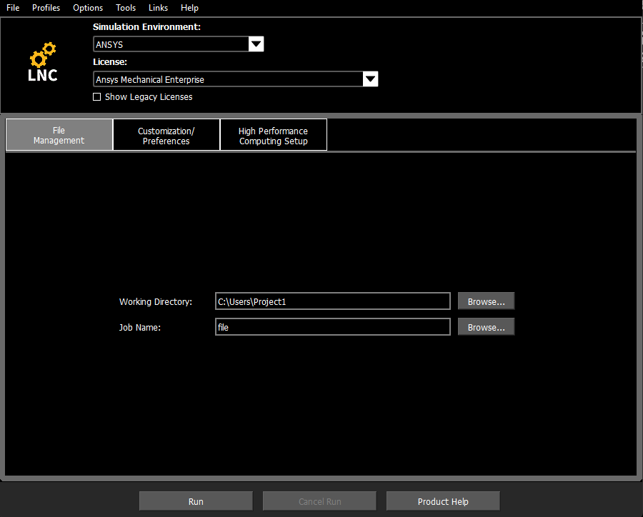
Job Name of the Launcher and /FILNAME
Product Launcher assigns the name with which the session is born. Template runs after
/FILNAME,m00_cantilever,1, so the main files of the exercise will use
m00_cantilever. Not a mistake: the script takes explicit control of your identity.
Step 3 — Become familiar with the MAPDL interface
Before running, take a minute to locate the main window and the Output Window:
Main window
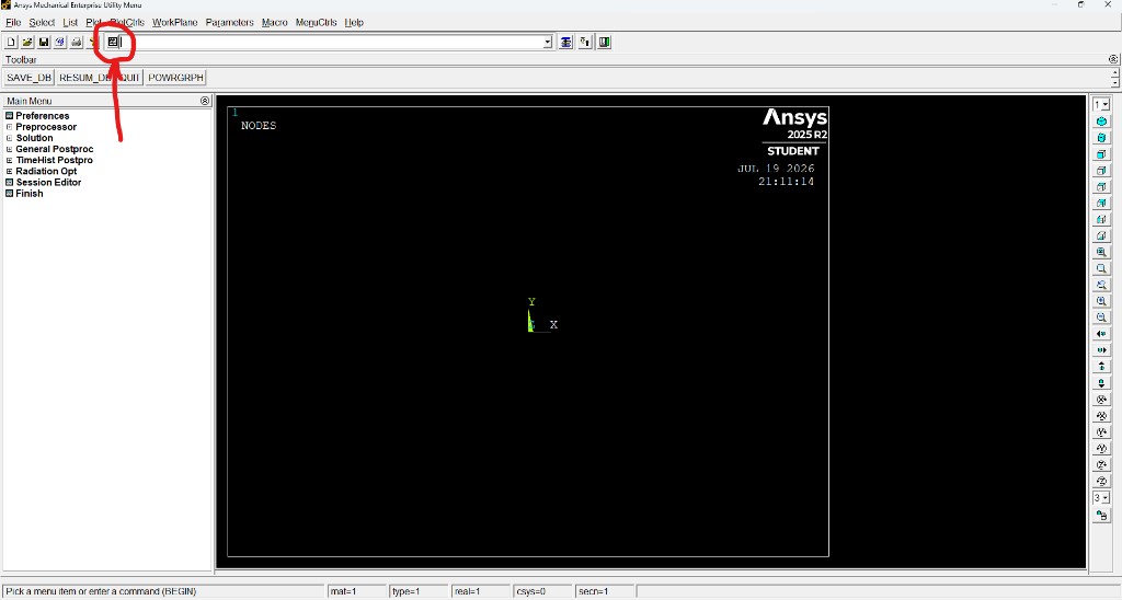
Five zones you'll use in almost every session:
- Command Input: top box where you can write an instruction.
- Main Menu: side tree with preprocessing, solution and postprocessing.
- viewport graphic area where geometry, mesh and results will appear.
- active processor in the bottom bar you will initially see
BEGIN. - Active Attributes:
mat,type,real,csysandsecnum.
Output Window
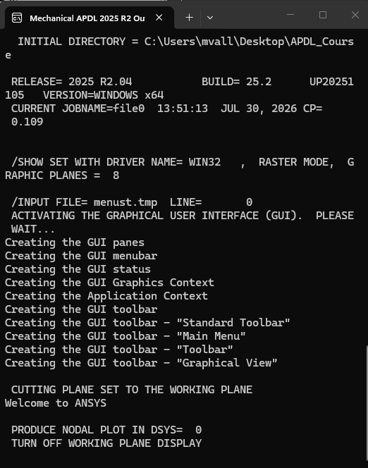
When you open MAPDL, a separate window entitled Mechanical APDL … Output. It is not where you type commands; it is the live log of everything the program writes — version and working directory, job name, graphical interface startup, command echo, solver progress, warnings, and errors.
On Windows, interactive MAPDL displays that output in the Output Window, but does not write it
to disk by default. To retain the log in a file, redirect it with
/OUTPUT,Fname,Ext or use the toolbar menu
Utility Menu → File → Switch Output to → File). In M00 it is not necessary to do it by hand:
/OUTPUT,m00_session,out is already included in the template, immediately
after /FILNAME.
The output file name must not match the job prefix. Because
/FILNAME sets m00_cantilever, and ANSYS reserves
m00_cantilever.out for the job, the template writes the execution log to the
alternative file m00_session.out.
While running, the Output Window remains the first place to spot an error; the
.out file lets you review the same content afterward.
BEGIN does not mean “without context”
BEGIN is the initial level of MAPDL: the session has just opened and you have not yet entered
no specific processor. A processor is the mode of work that determines what
APDL commands accept MAPDL at that time. Think of it as a phase of the analysis: not every
commands are valid in all phases.
The processors you'll use most often are four:
| Processor | Input (APDL) | What do you do on there? |
|---|---|---|
PREP7 |
/PREP7 |
Define geometry, materials, element types, mesh, and boundary conditions. |
SOLUTION |
/SOLU |
Declare the type of analysis and run SOLVE. |
POST1 |
/POST1 |
Read results and represent a spatial field in a set: contours, deformed, point listings. |
POST26 |
/POST26 |
Read results and represent a magnitude through several sets: load-response curves or temporal histories. |
POST1 and POST26 are complementary postprocessors: you enter one or the other after solving,
depending on whether you want to inspect a field in an instant or an evolution between sets. M00 template only uses
POST1; /POST26 you'll see it in M07.
To enter, type the command in Command Input and press Enter (or include it in a .mac).
To exit the current processor and return to BEGIN, use FINISH.
The bottom bar - the point 4 from the list above - shows where you are at all times; when running
the template you will see how it changes successively from BEGIN to PREP7,
SOLUTION and POST1.
The Main Menu of point 2 reflects the same logic: its preprocessing, solution and post-processing open those processors. In this course we will enter by APDL commands, not by menus.
Active attributes: defining is not activating
MAPDL uses numbered tables. ET,1,... defines the element type 1 and
MP,...,1,... defines the material 1. After TYPE,1 and MAT,1
turn them into active attributes for the elements to be created.
Pattern we will reuse: define → enable → assign when creating or meshing.
Step 4 — Undock the Command Window
Don't confuse the Output Window with the Command Window. The Output records all the session flow; the Command Window is optional and displays the interactive command dialog, immediate messages and responses. It can be integrated or decoupled depending on version and configuration.
Recommended settings during the course
Press the button indicated by the Red arrow in the previous screenshot to show the Command Window. If it is integrated into the interface, uncouple it and place it next to the viewport. It is not mandatory to solve, but it is highly recommended: you can follow the commands as execute and quickly detect the point at which a warning or error appears.
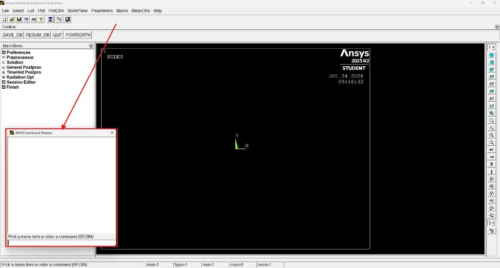
Use it as an interactive execution monitor, not as a substitute for on-disk recording. You don't need
read each line in real time or set up redirection by hand - template includes
/OUTPUT,m00_session,out pre-assigned and, in the end, a /OUTPUT without
arguments that returns the output to the Output Window in real time.
Step 5 — Run the template
Write in Command Input:
/INPUT,00_session_template,macThe instruction has three parts:
/INPUT: prompts MAPDL to read commands from a file.00_session_template: name without extension.mac.extension
If the file is in the Working Directory, you do not need to write the full path. During the execution you will see the geometry, the mesh and finally the contours appear.
INITIAL VERIFICATION
- Exist
m00_session.outandm00_cantilever.rston the Working Directory. - The Output Window does not end with a fatal error.
- An elongated beam is created in the X direction.
- The free end moves towards −Y.
- Displacement and stress contours are shown.
Physical model
The template represents a cantilever beam with the following characteristics:
| Magnitud | Value | Unit |
|---|---|---|
| Length | 1,00 | m |
| height | 0,10 | m |
| Width | 0,05 | m |
| Elastic modulus | 210·10⁹ | Pa |
| Poisson’s ratio | 0,30 | — |
| Total vertical force | −1000 | N |
The end x=0 is embedded and the load acts on the nodes of x=1 m.
The geometry is deliberately simple: at M00 we want to learn how to execute and read the analysis,
not solving a complicated geometry.
The same beam in the table and in the script
The table above fixes the physical problem. The APDL script translates each decision into commands.
These are not separate topics: each row corresponds to a section of the .mac file.
-
BLOCKBLOCK,0,1.0,0,0.10,0,0.050, 1.0— limits in X (length 1,0 m).0, 0.10— limits in Y (height 0,10 m).0, 0.05— limits in Z (width 0,05 m).
-
MP,EX,1,210E9
MP,PRXY,1,0.30EX,1,210E9— elastic modulus of the material 1 (Pa).PRXY,1,0.30— Poisson coefficient of the material 1.
-
D,ALL,ALL,0onx=0NSEL,S,LOC,X,0D,ALL,ALL,0NSEL,S,LOC,X,0— select the nodes in the planex=0.D,ALL,ALL,0— constrains all degrees of freedom in the current selection.
-
F,ALL,FY,-1000/n_tipNSEL,S,LOC,X,1.0*GET,n_tip,NODE,0,COUNTF,ALL,FY,-1000/n_tipNSEL,S,LOC,X,1.0— select the nodes on the free end.*GET,n_tip,...— counts how many nodes are selected.F,ALL,FY,-1000/n_tip— distributes −1000 N among those nodes in Y.
When reading the anatomy of the script, do not memorize single lines: locate which physical decision encodes each block. Hover your cursor (or focus) over ? to view the command and the meaning of each argument.
Script anatomy
Opens the file in an editor. It is divided into five blocks:
- Initialize Database
- Define and mesh the model.
- Apply underlayment and load.
- Overcome
- Read and represent results.
Block 1 — Initialize the session
/CLEAR,START
/FILNAME,m00_cantilever,1
/OUTPUT,m00_session,out
/TITLE,M00 - Cantilever beam
/UNITS,SI| Command | Function | Verification |
|---|---|---|
/CLEAR,START | Clean the database and reread the initial settings. | The session returns to BEGIN. |
/FILNAME | Defines the base name of the exercise files. | Files start with m00_cantilever. |
/OUTPUT,m00_session,out | Redirects text output to a file other than the one reserved for the job. | After /INPUT, m00_session.out appears in the working directory. |
/TITLE | Assign a descriptive title to the model. | Appears in supported listings and charts. |
/UNITS,SI | Documents the unit convention. | It does not convert any value. |
Order matters.
/CLEAR appears before the title and the units because it restarts the database.
/FILNAME sets the job prefix (m00_cantilever) and booking
m00_cantilever.outThat’s why. /OUTPUT,m00_session,out goes right away with
an alternate name. You don't have to repeat these commands or use the Switch Output to menu on M00.
Block 2 — Enter PREP7 and define attributes
/PREP7
ET,1,SOLID185
MP,EX,1,210E9
MP,PRXY,1,0.30
TYPE,1
MAT,1/PREP7enters the preprocessor: geometry, elements, materials, mesh and conditions.ET,1,SOLID185defines the element type 1 as a structural solid.MP,EX,1,210E9defines the elastic modulus of the 1 material.MP,PRXY,1,0.30defines its Poisson coefficient.TYPE,1andMAT,1activate those boards before meshing.
M03 will justify in detail the choice of the element and compare idealizations. In M00 just recognize which element and material must be defined and active before generating elements.
Block 3 — Create geometry and mesh
BLOCK,0,1.0,0,0.10,0,0.05
ESIZE,0.025
VMESH,ALLBLOCKcreates a rectangular volume with X, Y and Z boundaries.ESIZEproposes an overall element size.VMESH,ALLmesh all selected volumes.
A visible mesh does not imply a converged mesh. M04 will study sensitivity and quality. Here we only need reasonable discretization to complete the flow.
Block 4 — Select and constrain
NSEL,S,LOC,X,0
D,ALL,ALL,0
ALLSEL,ALL
NSEL,S,LOC,X,0 replaces the current selection with the nodes located in x=0.
D,ALL,ALL,0 restricts all of its available degrees of freedom. Finally,
ALLSEL,ALL retrieves all entities.
Selection is status
Many commands act only on the selected one. Forget ALLSEL can make stages
ignoring much of the model without the problematic line appearing incorrect.
Block 5 — Distribute the total force
NSEL,S,LOC,X,1.0
*GET,n_tip,NODE,0,COUNT
F,ALL,FY,-1000/n_tip
ALLSEL,ALL
The end nodes are selected first. *GET count how many there are and save the result
en n_tip. The strength of each node is -1000/n_tip, so the sum remains
equal to − 1000N even if you change the mesh.
This idea is important: the input value represents a total force, not a force that must be repeated in full at each node.
Block 6 — Exit PREP7 and Solve
FINISH

/SOLU
ANTYPE,STATIC
SOLVE
FINISHFINISHexits the current processor and returns to BEGIN./SOLUgoes into Solution.ANTYPE,STATICdeclares a static analysis.SOLVErequests the solution of the current load step.- The second
FINISHcloses the solution stage.
That SOLVE finish only proves that the solver got an answer. We still have to
check if it correctly represents the physical problem.
Block 7 — Enter POST1
/POST1
SET,LAST
PLNSOL,U,SUM
PLNSOL,S,EQV
FINISH

/OUTPUT/POST1opens the general postprocessor.SET,LASTread the latest set of results available.PLNSOL,U,SUMrepresents the magnitude of the displacement.PLNSOL,S,EQVrepresents the equivalent stress./OUTPUTwith no arguments returns live text output to the Output Window.
Each plot replaces the previous one in the viewport. At the end you will see the equivalent stress.
You can rerun PLNSOL,U,SUM manually to restore the displacement contour.
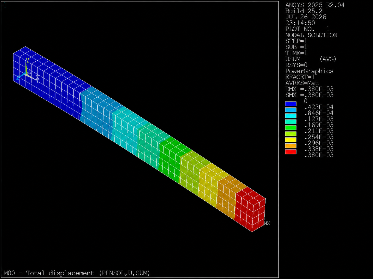
PLNSOL,U,SUM). It connects the model to its results; it does not demonstrate convergence or analytical validation.
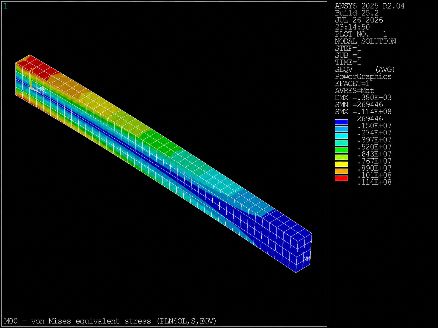
PLNSOL,S,EQV). A second type of visual inspection; it does not replace the linearity challenge tolerances.
What files should you find
| Public records | What’s on | Why It Matters |
|---|---|---|
m00_session.out | Text log from /OUTPUT,m00_session,out until the later /OUTPUT command. | Diagnostics and a reproducible trace of the script. |
m00_cantilever.out | Output associated with the job name (/FILNAME). | MAPDL reserves it with that name; in M00 the useful record of the script is in m00_session.out. |
m00_cantilever.rst | Structural Results | Allows post-processing. |
m00_cantilever.log Session log | Commands sent during the session. | Helps rebuild actions. |
m00_cantilever.db | Model database on disk. | The M00 template does not run SAVE; do not expect this file unless you save it yourself. |
If you run the template multiple times (for example, in the linearity challenge), the file
m00_session.out is overwritten at each run. Files may also appear
with numbered job names such as m00_cantilever1.out when
/FILNAME,...,1 opens a new record. For script diagnosis, use
m00_session.out of the execution you just completed.
How to read the .out file
The template includes /OUTPUT,m00_session,out immediately after
/FILNAME. From there, what MAPDL writes in the Output Window also remains in
m00_session.out until the final /OUTPUT, which returns output to the
live window. Open it as text and search,
in this order:
ERRORorFATAL: may invalidate or stop the execution.WARNING: Requires interpretation; not all warnings are of equal severity.- The solution section: confirms that it was reached
SOLVE. - The end of the file: check that the script reached
POST1.
Do not change solver options at random at the first message. Identify the stage first, the entity and instruction related to the symptom.
Independent physical check
For a rectangular beam:
I = B·H³/12
|uy_tip| = P·L³/(3·E·I)
With the model values:
I = 4.1667E-6 m⁴
|uy_tip| ≈ 3.81E-4 m = 0.381 mm
The 3D solid model does not have to match Euler–Bernoulli exactly. In this first session we look for the order of magnitude. M04 and M07 will turn this comparison into a formal study.
Verifiable challenge — The linearity test
Before modifying anything, predict what will happen when the load is duplicated:
F,ALL,FY,-2000/n_tip- Run the case of −1000 N and record the vertical displacement of the end.
- Only change the total force to −2000 N.
- Run again with the same geometry, material and mesh.
- Compute
uy_2000/uy_1000.
Acceptance criterion: ratio between 1.99 and 2.01.
In a linear elastic analysis, doubling the load doubles displacements and stresses. The ratio is more informative than comparing two contour screenshots.
Common mistakes
| Symptom | Likely cause | Check |
|---|---|---|
File not found | The `.mac` is not in Working Directory. | Check folder and name in `/INPUT`. |
| Division by zero | No nodes found in x=1.0. | Review geometry, mesh and selection. |
| No contours | There is no valid result set. | Look for SOLVE errors in m00_session.out. |
| Displacement toward +Y | The load sign changed. | Review FY and its sign. |
| Gigantic displacement | Inconsistent units. | Check meters, newtons and pascals. |
| Only part of the model appears | Residual selection. | Run ALLSEL,ALL. |
What we have chosen to postpone
M00 does not use local coordinate systems, work plane, loads on element faces
or SFCONTROL. They are valid tools, but introducing them here would hide the essential workflow.
We simplify the model, not the explanation. Each concept will appear when solving a problem that the student already recognizes.
Self-assessment
What is the difference between Working Directory and Job Name?
Working Directory indicates where files are read and written; Job Name sets its initial prefix.
What does BEGIN indicate?
That MAPDL is at the initial level, outside of PREP7, SOLUTION, POST1 or POST26.
Why do TYPE, 1and MAT, 1appear before VMESH?
Because first the tables are defined and then the attributes that the elements will receive when meshing are activated.
Why do we divide −1000 by n_tip?
So that the total force remains the same even if the number of end nodes changes.
Does SOLVE without errors prove that the model is correct?
No. Conditions must still be checked, deformed, equilibrium, order of magnitude and sensitivity.
/UNITS converts millimeters to meters?
No. It documents the convention used, but numerical consistency remains the responsibility of the user.
Evidence of learning
- Working Directory
00_session_template.mac,m00_session.outandm00_cantilever.rst. - A viewport screenshot showing the deformed shape or displacement contour.
- An excerpt from
m00_session.outconfirming that the solution completed. - Table with load, displacement and ratio between the two cases.
- A brief explanation of why the observed ratio demonstrates linear behavior.
Validation checklist
- I created a dedicated folder with write permissions.
- I set up Working Directory and Job Name on Product Launcher.
- I identified Command Input, Output Window, Command Window, viewport, processor and attributes.
- Execute the template using
/INPUT. - I found
m00_session.outandm00_cantilever.rst. - The deformation and direction of travel are physically reasonable.
- I compared the order of magnitude to
0.381 mm. - I completed the challenge with a ratio between
1.99and2.01. - I can explain the function of each block of the script without memorizing all its arguments.
Next
You already know how to open, run and check a reproducible simulation. In M01 you will convert their numbers fixed in parameters, you will add validations and have the program make its first design decision.