When a bearing inner race is press-fitted onto a shaft, radial interference creates contact pressure and stresses in both parts. This note walks through an APDL model of that assembly: what it represents, how to run it in Mechanical APDL, and what each block of the script does.
Step 1 — The physical problem
The model represents a solid shaft (50 mm diameter) and a bearing inner race (50 mm bore, 60 mm OD) with 0.5 mm radial interference. Steel properties (E = 206 GPa, ν = 0.3) and a static nonlinear contact solve reproduce the press-fit state.
- Shaft outer radius: 25 mm (nominal)
- Bearing inner radius: 25 mm (nominal)
- Radial interference GAP: 0.5 mm via contact surface offset
- Quarter section (0–90°) with symmetry BCs
Step 2 — Open MAPDL and run the script
Launch Mechanical APDL, set the working directory to the folder containing the macro, and run:
/INPUT,bearing_shaft_interference,macDownload bearing_shaft_interference.mac
The script runs in one pass through /PREP7 → /SOLUTION → /POST1. You can also paste blocks individually while learning each stage.
Step 3 — Geometry (/PREP7)
Parameters IR_SHAFT, OR_SHAFT, IR_BEARING, OR_BEARING and WIDTH define the assembly. Two CYLINDER commands create the shaft and inner race; only a 90° wedge is meshed to exploit symmetry.
CYLINDER,IR_SHAFT,OR_SHAFT,0,WIDTH,0,90
CYLINDER,IR_BEARING,OR_BEARING,0,WIDTH,0,90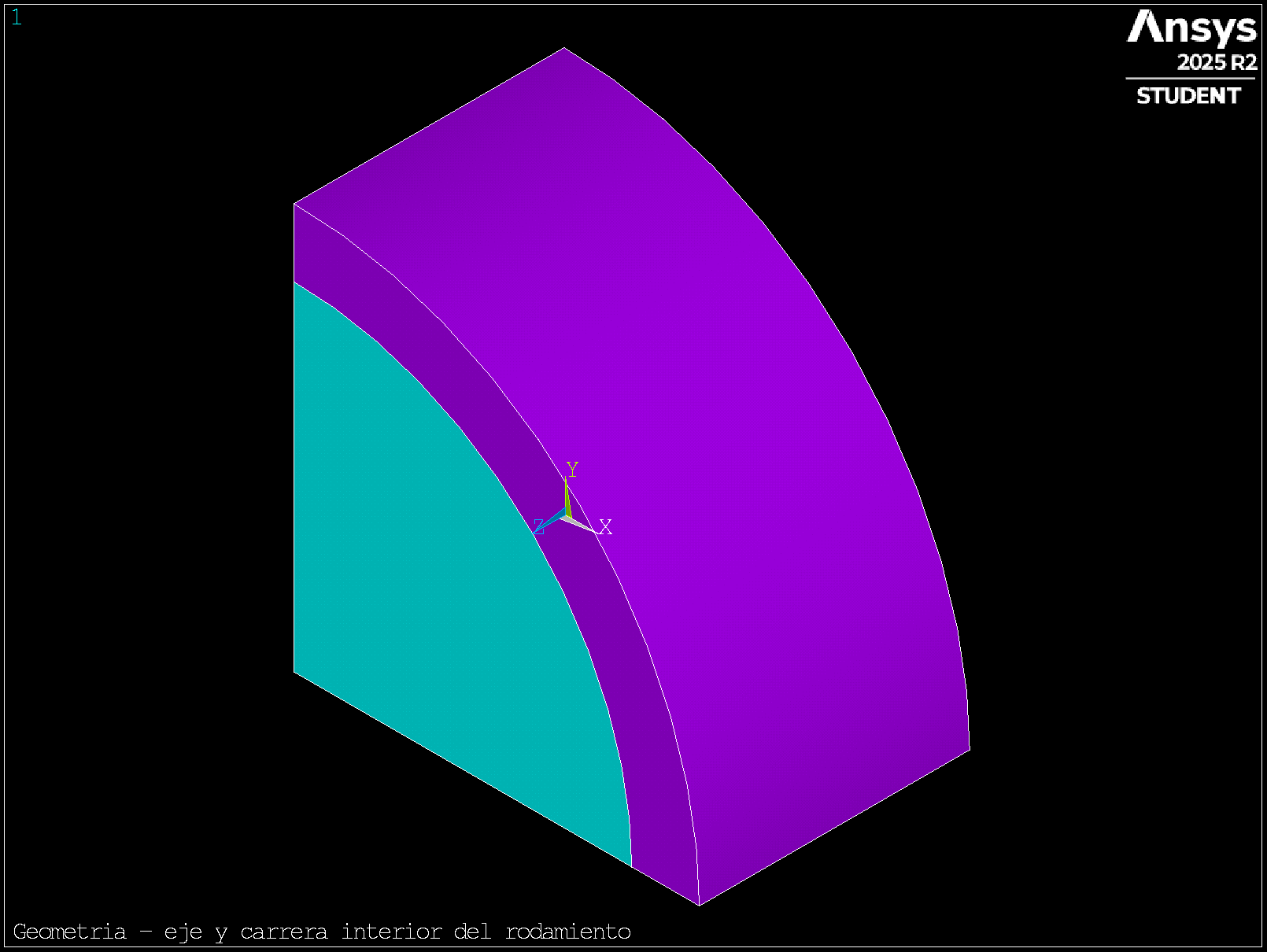
Step 4 — Mesh
SOLID185 hexahedra with ESIZE = 0.002 m (2 mm). Refine this value if contact pressure or stresses need a mesh convergence study.
ET,1,SOLID185
ESIZE,0.002
VMESH,ALL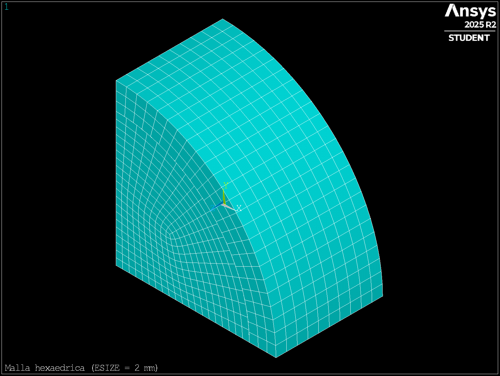
Step 5 — Contact with interference
A CONTA174 / TARGE170 pair models the shaft–bearing interface. The key line is RMODIF,2,10,GAP: it applies a 0.5 mm contact offset so the bearing bore starts inside the shaft surface, simulating press-fit interference without changing the nominal CAD dimensions.
RMODIF,2,10,GAP    ! offset radial = interferencia
CSYS,1
ASEL,S,LOC,X,IR_BEARING    ! superficie de contacto
...
ASEL,S,LOC,X,OR_SHAFT       ! superficie target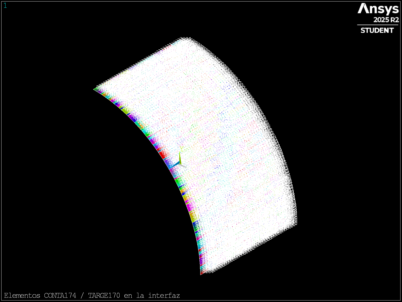
Step 6 — Boundary conditions and SOLVE
Symmetry on the Y = 0 and Y = 90 planes (cylindrical CSYS) and fixed axial faces at Z = 0 and Z = WIDTH. The static solve uses ramped loading (KBC,0) so contact closes gradually.
/SOLUTION
ANTYPE,STATIC
KBC,0
NSUBS,1,10,1
SOLVE
Step 7 — Contact pressure (/POST1)
After SET,LAST, plot PLESOL,CONT,PRES on the contact elements. This is the primary quantity for checking whether the fit is too tight or too loose.
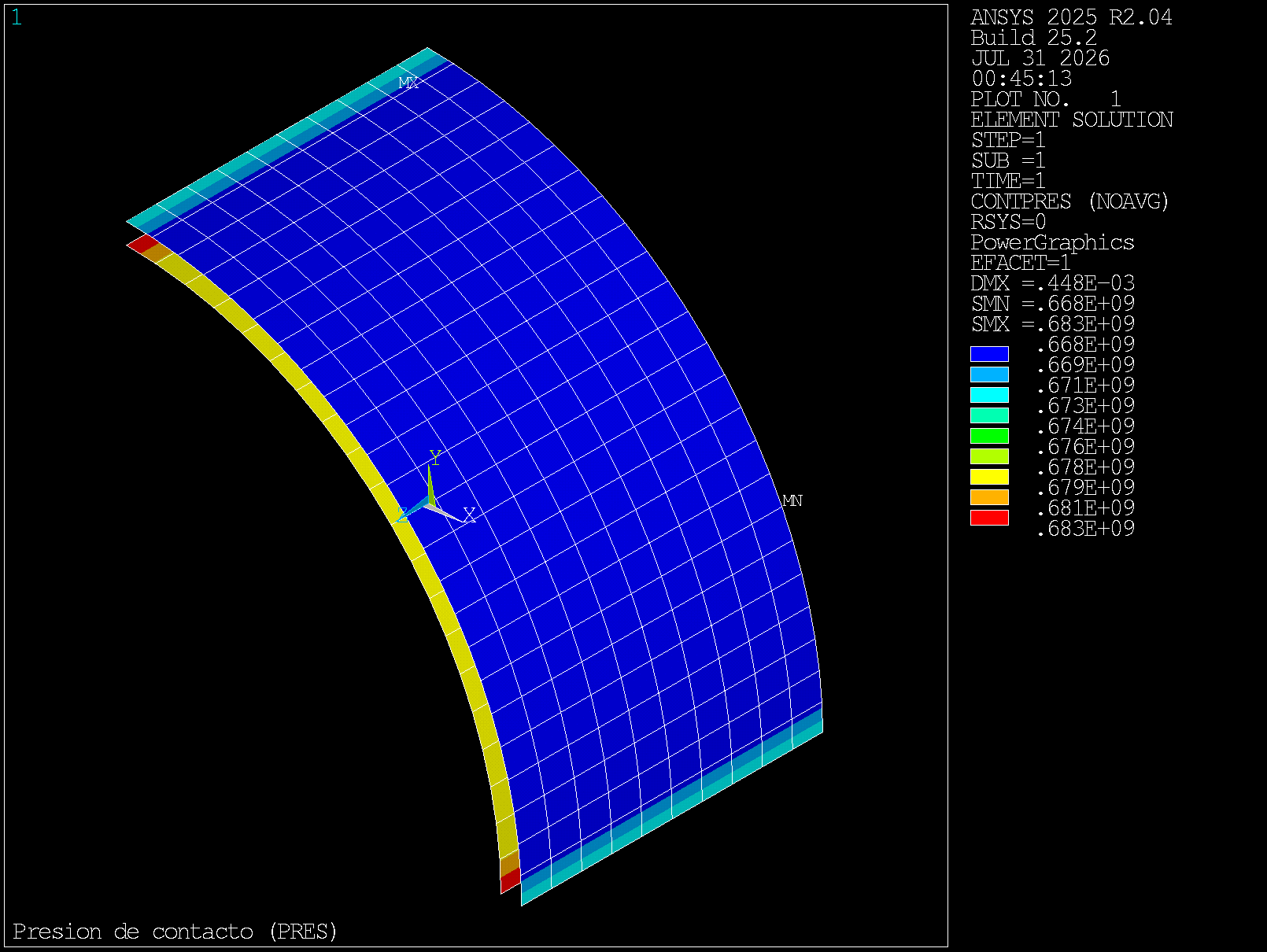
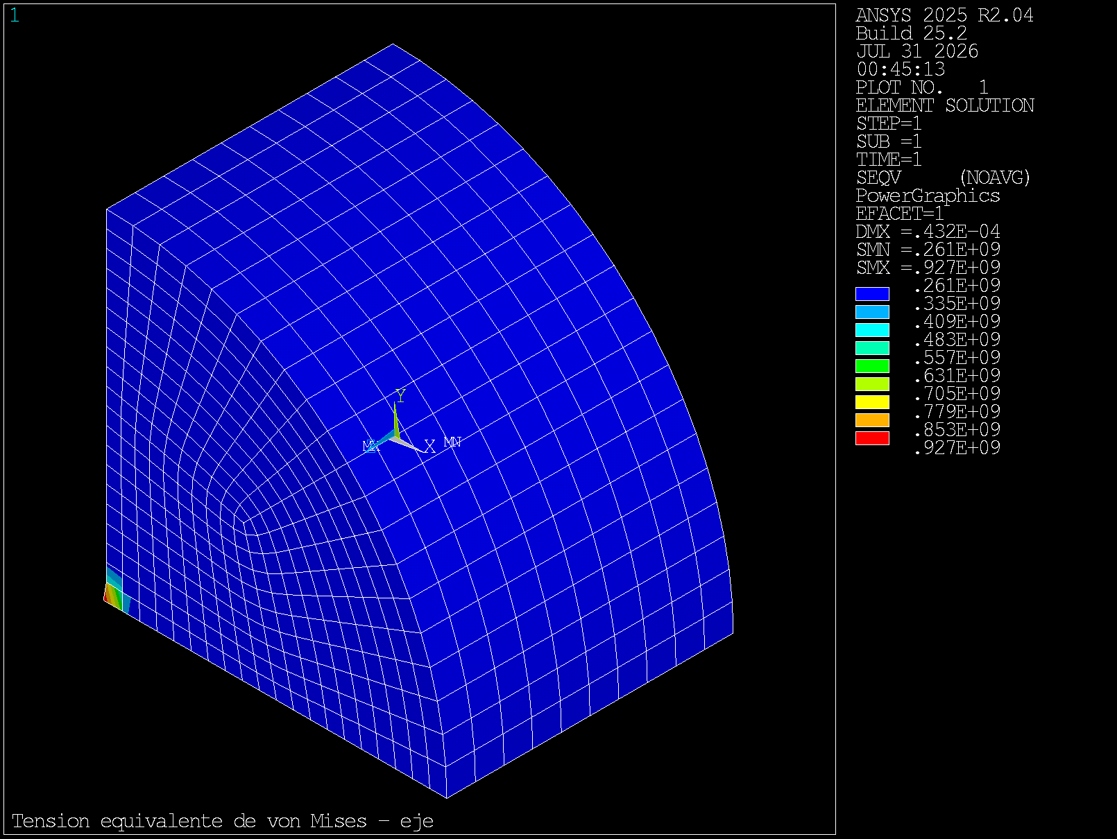
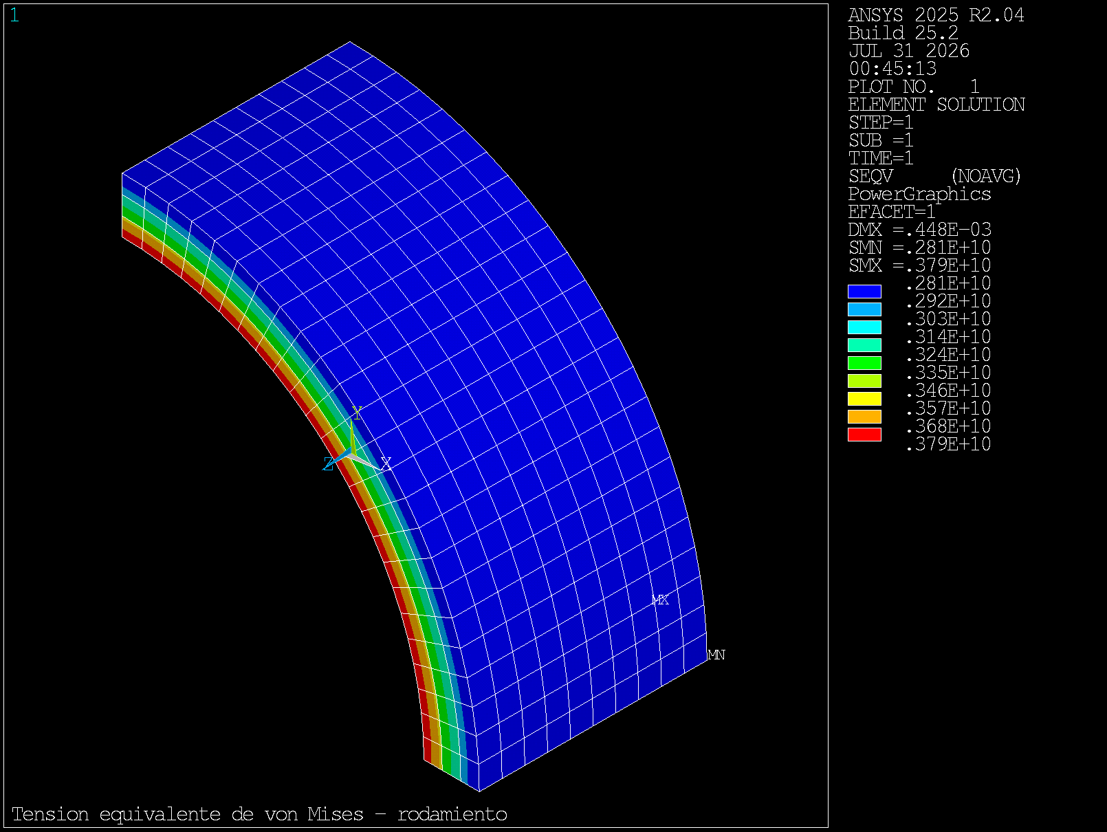
Step 8 — von Mises stress in both parts
PLESOL,S,EQV on the shaft volume and on the bearing inner race reveals stress concentrations that could drive cracking during assembly or service.
Step 9 — Compare with the analytical solution
The script computes classical thick-cylinder press-fit pressure and compares it with the MAPDL peak. Use this ratio as a mesh and model sanity check.
Pressure 629444444.444 3790536960.000 0.166Example with ESIZE = 2 mm on Ansys Student 2025 R2. Refine the mesh at the interface for closer agreement.
Troubleshooting
| Problem | What to do |
|---|---|
| File not found on /INPUT | Confirm bearing_shaft_interference.mac is in the working directory (File → Change Directory or /PWD). |
| SOLVE fails or contact does not close | Check GAP matches the intended radial interference and that cylindrical selections in CSYS,1 hit the correct radii. |
| No contours appear | Enter /POST1, run SET,LAST, then PLESOL or PLNSOL on the selected entities. |
| Large analytical vs MAPDL gap | Reduce ESIZE near the interface and repeat the solve. |
In mechanical design, geometric interferences are a common and critical phenomenon that can determine the success or failure of an assembly. When a bearing is mounted on a shaft with interference, a complex stress state is generated that, if not properly analyzed, can lead to premature failures, cracks, or even catastrophic fractures.
Finite element simulation (FEA) allows us to predict and anticipate these problems before they occur in reality, saving time, costs, and avoiding safety risks. In this resource, we present a complete Ansys APDL script to simulate the contact pressure between a shaft and a bearing during interference fit assembly.
Why is it important to simulate geometric interferences?
Geometric interferences occur when two components are assembled with dimensions that generate an initial contact pressure. This phenomenon is intentional in many cases (such as in press fits) but can be problematic if not properly controlled.
Benefits of simulation
- Stress prediction: Identify areas of high stress concentration that could lead to fatigue or overload failures.
- Design optimization: Adjust tolerances and dimensions to achieve the optimal fit without compromising structural integrity.
- Material validation: Verify that selected materials can withstand the stresses generated during assembly and in service.
- Prototype reduction: Minimize the need for costly and destructive physical testing.
- Problem anticipation: Detect possible cracks, fractures, or excessive deformations before manufacturing.
The case study: bearing-shaft
In this example, we simulate the assembly of a bearing on a shaft with geometric interference. The Ansys APDL script models:
- • Solid shaft: Nominal outer radius of 25 mm (50 mm diameter)
- • Bearing (inner race): Nominal inner radius of 25 mm, outer radius of 30 mm
- • Radial interference: 0.5 mm (applied via contact surface offset)
- • Material: Steel (E = 206 GPa, ν = 0.3)
- • Analysis: Nonlinear static with contact
The script uses contact elements (CONTA174/TARGE170) to model the interaction between the shaft and bearing, applying the interference through an offset on the contact surface. This allows simulating the real stress state generated during assembly.
Ansys APDL Script
Below is the complete script for Ansys APDL. This script includes:
- • Geometry and parameter definition
- • Material properties
- • Automatic meshing
- • Contact definition with interference
- • Boundary conditions and symmetry
- • Solution and post-processing
- • Comparison with analytical solution
Ansys APDL Script - Geometric Interference Simulation
APDL/TITLE,INTERFERENCE FIT BETWEEN BEARING AND SHAFT
/COM, ============================================================
/COM, SIMULACION DE INTERFERENCIA GEOMETRICA: RODAMIENTO-EJE
/COM, ============================================================
/COM,
/COM, Este ejemplo demuestra la importancia de modelar interferencias
/COM, geometricas en el diseno mecanico. Cuando un rodamiento se
/COM, introduce en un eje con interferencia geometrica, se genera un
/COM, estado tensional tanto en el eje como en el rodamiento.
/COM, ============================================================
FINISH
/CLEAR
/OUT,SCRATCH
/PREP7
! ============================================================
! GEOMETRIC PARAMETERS - BEARING-SHAFT ASSEMBLY
! ============================================================
! Dimensions in meters (can be adjusted for different scales)
! Typical bearing-shaft assembly dimensions
IR_SHAFT = 0.0 ! INNER RADIUS OF SHAFT (SOLID SHAFT = 0)
OR_SHAFT = 0.025 ! OUTER RADIUS OF SHAFT (50mm DIAMETER - NOMINAL)
IR_BEARING = 0.025 ! INNER RADIUS OF BEARING INNER RACE (50mm DIAMETER - NOMINAL)
OR_BEARING = 0.030 ! OUTER RADIUS OF BEARING INNER RACE
WIDTH = 0.020 ! WIDTH OF THE ASSEMBLY IN M (20mm)
GAP = 0.0005 ! INTERFERENCE IN M (0.5mm RADIAL INTERFERENCE)
! NOTE: Geometry uses nominal dimensions. Interference
! is applied via contact surface offset (RMODIF,2,10,GAP)
! ============================================================
! MATERIAL PROPERTIES
! ============================================================
! Steel properties for both shaft and bearing
E = 206E9 ! YOUNG'S MODULUS IN N/M^2 (STEEL)
NU = 0.3 ! POISSON'S RATIO (STEEL)
MP,EX,1,E
MP,NUXY,1,NU
! ============================================================
! ELEMENT TYPE
! ============================================================
ET,1,SOLID185 ! SOLID185 ELEMENTS (3D SOLID)
! ============================================================
! CREATE GEOMETRY
! ============================================================
! Create shaft (inner cylinder)
CYLINDER,IR_SHAFT,OR_SHAFT,0,WIDTH,0,90
! Create bearing inner race (outer cylinder)
CYLINDER,IR_BEARING,OR_BEARING,0,WIDTH,0,90
! ============================================================
! MESHING
! ============================================================
ESIZE,0.002 ! ELEMENT SIZE (2mm)
TYPE,1
MAT,1
VMESH,ALL ! MESHING CYLINDERS
ALLSEL,ALL
! ============================================================
! CONTACT DEFINITION
! ============================================================
! Define contact pair between shaft and bearing
SECTYPE,2,CONTACT,CYLINDER
SECDATA,0,0,0,0,0,2.00 ! GEOMETRY CORRECTION FOR CYLINDER
ET,2,CONTA174 ! CONTA174 ELEMENTS (CONTACT SURFACE)
ET,3,TARGE170 ! TARGE170 ELEMENTS (TARGET SURFACE)
REAL,2
KEYOPT,2,2,0 ! AUGMENTED LAGRANGE ALGORITHM
KEYOPT,2,12,0 ! STANDARD CONTACT
KEYOPT,2,10,0 ! ITERATION BASED CONTACT STIFFNESS UPDATE
KEYOPT,2,4,3 ! PROJECTION BASED METHOD
KEYOPT,2,9,2 ! INCLUSION OF GEOMETRICAL PENETRATION WITH RAMPED EFFECTS
R,2
RMODIF,2,10,GAP ! CONTACT SURFACE OFFSET (INTERFERENCE)
! ============================================================
! CREATE CONTACT ELEMENTS
! ============================================================
! Contact surface on bearing inner race
! Note: Area numbers may vary. If ASEL by area number fails,
! use selection by location: ASEL,S,LOC,X,IR_BEARING
TYPE,2
REAL,2
SECNUM,2
CSYS,1 ! CYLINDRICAL COORDINATE SYSTEM
ASEL,S,LOC,X,IR_BEARING ! SELECT BEARING INNER SURFACE BY RADIUS
NSLA,S,1
ESLN,S
ESURF ! FORMING CONTACT ELEMENTS
ALLSEL,ALL
! Target surface on shaft outer surface
TYPE,3
REAL,2
CSYS,1 ! CYLINDRICAL COORDINATE SYSTEM
ASEL,S,LOC,X,OR_SHAFT ! SELECT SHAFT OUTER SURFACE BY RADIUS
NSLA,S,1
ESLN,S
ESURF ! FORMING TARGET ELEMENTS
ALLSEL,ALL
CSYS,0 ! RETURN TO CARTESIAN COORDINATE SYSTEM
! ============================================================
! BOUNDARY CONDITIONS
! ============================================================
! Apply symmetry conditions
CSYS,1 ! CYLINDRICAL COORDINATE SYSTEM
! Constrain radial displacement at symmetry plane (Y=0)
NSEL,S,LOC,X,IR_SHAFT,OR_BEARING
NSEL,R,LOC,Y,0
D,ALL,UY,0 ! CONSTRAINING UY DOF (RADIAL)
ALLSEL,ALL
! Constrain tangential displacement at symmetry plane (Y=90)
NSEL,S,LOC,Y,90,90
D,ALL,UX,0 ! CONSTRAINING UX DOF (TANGENTIAL)
ALLSEL,ALL
! Constrain axial displacement at front and back faces
NSEL,S,LOC,Z,0
NSEL,A,LOC,Z,WIDTH
D,ALL,UZ,0 ! CONSTRAINING UZ AT FRONT AND BACK FACES
ALLSEL,ALL
FINISH
! ============================================================
! SOLUTION
! ============================================================
/SOLUTION
ANTYPE,STATIC ! PERFORM STATIC ANALYSIS
OUTRES,ALL,ALL
TIME,1.0
KBC,0 ! RAMPED LOADING
NSUBS,1,10,1
SOLVE
FINISH
! ============================================================
! POST-PROCESSING
! ============================================================
/POST1
SET,LAST
/OUT,
/COM, ============================================================
/COM, ANALYTICAL SOLUTION FOR INTERFERENCE FIT
/COM, ============================================================
IR12 = IR_SHAFT*IR_SHAFT
OR12 = OR_SHAFT*OR_SHAFT
OR22 = OR_BEARING*OR_BEARING
OR13 = OR_SHAFT*OR_SHAFT*OR_SHAFT
TERM1 = ((OR22-OR12)*(OR12-IR12))/(OR22-IR12)
TERM2 = (E*GAP)/(2*OR13)
PRES = TERM2*TERM1
/COM,
/COM, ANALYTICAL CONTACT PRESSURE: PRES = ,PRES, Pa
/COM,
! ============================================================
! VISUALIZATION
! ============================================================
/OUT,SCRATCH
/VIEW,1,1,1,1
/GRAPHICS,POWER
! Plot contact pressure
ESEL,S,ENAME,,174
PLESOL,CONT,PRES
ESEL,ALL
! Select nodes at contact interface for detailed view
VSEL,S,VOLUME,,2,,,1
NSEL,R,LOC,X,OR_SHAFT
NSEL,R,LOC,Y,40,60
ESLN,S
ESEL,R,ENAME,,174
PLESOL,CONT,PRES
*GET,PRESMAX,PLNSOL,0,MAX
*GET,PRESMIN,PLNSOL,0,MIN
ALLSEL,ALL
/SHOW,CLOSE
/OUT,
*STAT,PRESMAX
*STAT,PRESMIN
! ============================================================
! STRESS ANALYSIS
! ============================================================
! Plot von Mises stress in shaft
VSEL,S,VOLUME,,1
NSLV,S,1
ESLV,S
PLESOL,S,EQV
ALLSEL,ALL
! Plot von Mises stress in bearing
VSEL,S,VOLUME,,2
NSLV,S,1
ESLV,S
PLESOL,S,EQV
ALLSEL,ALL
! Plot radial stress
PLESOL,S,X
ALLSEL,ALL
! Plot hoop stress
PLESOL,S,Y
ALLSEL,ALL
! ============================================================
! RESULTS COMPARISON
! ============================================================
/OUT,SCRATCH
*DIM,LABEL,CHAR,1,2
*DIM,VALUE,,1,3
LABEL(1,1) = 'Pressure'
*VFILL,VALUE(1,1),DATA,PRES ! FROM ANALYTICAL SOLUTION
*VFILL,VALUE(1,2),DATA,PRESMAX ! FROM MAPDL
*VFILL,VALUE(1,3),DATA,ABS(PRES/PRESMAX)! RATIO
/COM,
/COM,
/OUT,bearing_shaft_results,vrt
/COM,-----------------BEARING-SHAFT INTERFERENCE RESULTS----------------
/COM,
/COM, | ANALYTICAL | Mechanical APDL | RATIO
/COM,
/COM,
*VWRITE,LABEL(1,1),VALUE(1,1),VALUE(1,2),VALUE(1,3)
(1X,A17,' ',F15.3,' ',F15.3,' ',F5.3)
/COM,
/COM,
/COM,------------------------------------------------------------------
/OUT,
*LIST,bearing_shaft_results,vrt
FINISH
Main features of the script
1. Geometry modeling
The script creates two cylinders representing the shaft and bearing. It uses a quarter section (0-90 degrees) taking advantage of symmetry conditions to reduce model size and computation time.
2. Contact definition with interference
The interference is applied through the command RMODIF,2,10,GAP, which sets an offset on the contact surface. This simulates the forced assembly of the bearing onto the shaft.
3. Boundary conditions
Symmetry conditions are applied on planes Y=0 and Y=90, and axial constraints on the front and back faces. This allows correctly modeling the behavior of the complete assembly using only a quarter of the model.
4. Validation with analytical solution
The script includes the calculation of contact pressure using classical analytical formulas for press fits, allowing comparison of numerical results with the theoretical solution and model validation.
Results interpretation
Once the script is executed, the main results to analyze are:
Key parameters to evaluate
- • Contact pressure: Verify that it does not exceed material limits and is sufficient to ensure the fit.
- • Von Mises stress: Identify areas of high stress concentration that could lead to failures.
- • Radial and hoop stress: Analyze the stress distribution in both components.
- • Analytical comparison: Validate that numerical results match the theoretical solution.
Important considerations
Points of attention
- The script uses a simplified model (quarter section). For more complex cases, it may be necessary to model the complete geometry.
- Material properties assume linear elastic behavior. For more accurate analyses, consider including plasticity or nonlinear effects.
- The interference is applied via contact offset. Ensure that the GAP value is consistent with actual manufacturing tolerances.
- The mesh must be sufficiently fine in the contact zone to correctly capture local stresses.
Conclusion
The simulation of geometric interferences through finite elements is an essential tool in modern mechanical design. It allows predicting and anticipating problems that would otherwise only be discovered during physical testing or, worse, during component service.
If you need to adapt this script to your specific case or have questions about results interpretation, do not hesitate to contact us. We specialize in finite element analysis and can help you optimize your designs through numerical simulation.